Prediction of Confidence Rating and Reaction Time Distribution in race models of confidence
Source:R/predictratingdist_RM.R
predictRM.RdpredictRM_Conf predicts the categorical response distribution of
decision and confidence ratings, predictRM_RT computes the
RT distribution (density) in the independent and partially anti-correlated
race models (Hellmann et al., 2023), given specific parameter
constellations. See RaceModels for more information about the models
and parameters.
Usage
predictRM_Conf(paramDf, model = "IRM", time_scaled = FALSE, maxrt = Inf,
  subdivisions = 100L, stop.on.error = FALSE, .progress = TRUE)

predictRM_RT(paramDf, model = "IRM", time_scaled = FALSE, maxrt = 9,
  subdivisions = 100L, minrt = NULL, scaled = FALSE, DistConf = NULL,
  .progress = TRUE)
Arguments
- paramDf
a list or data frame with one row. Column names should match the names of RaceModels parameter names (only
mu1andmu2are not used in this context but replaced by the parameterv). For different stimulus quality/mean drift rates, names should bev1,v2,v3,.... Differentsparameters are possible withs1,s2,s3,... with equally many steps as for drift rates. Additionally, the confidence thresholds should be given by names withthetaUpper1,thetaUpper2,...,thetaLower1,... or, for symmetric thresholds only bytheta1,theta2,....- model
character scalar. One of "IRM" or "PCRM". ("IRMt" and "PCRMt" will also be accepted. In that case, time_scaled is set to TRUE.)
- time_scaled
logical. Whether the confidence measure should be scaled by 1/sqrt(rt). Default: FALSE. (It is set to TRUE, if model is "IRMt" or "PCRMt")
- maxrt
numeric. The maximum RT for the integration/density computation. Default: 15 (for
predictRM_Conf(integration)), 9 (forpredictRM_RT).- subdivisions
integer(default: 100). ForpredictRM_Confit is used as argument for the inner integral routine. ForpredictRM_RTit is the number of points for which the density is computed.- stop.on.error
logical. Argument directly passed on to integrate. Default is FALSE, since the densities invoked may lead to slow convergence of the integrals (which are still quite accurate) which causes R to throw an error.
- .progress
logical. If TRUE (default) a progress bar is drawn to the console.
- minrt
numeric or NULL(default). The minimum rt for the density computation.
- scaled
logical. For
predictRM_RT. Whether the computed density should be scaled to integrate to one (additional columndensscaled). Otherwise the output contains only the defective density (i.e. its integral is equal to the probability of a response and not 1). IfTRUE, the argumentDistConfshould be given, if available. Default:FALSE.- DistConf
NULLordata.frame. Adata.frameormatrixwith column names, giving the distribution of response and rating choices for different conditions and stimulus categories in the form of the output ofpredictRM_Conf. It is only necessary, ifscaled=TRUE, because these probabilities are used for scaling. Ifscaled=TRUEandDistConf=NULL, it will be computed with the functionpredictRM_Conf, which takes some time and the function will throw a message. Default:NULL
Value
predictRM_Conf returns a data.frame/tibble with columns: condition, stimulus,
response, rating, correct, p, info, err. p is the predicted probability of a response
and rating, given the stimulus category and condition. info and err refer to the
respective outputs of the integration routine used for the computation.
predictRM_RT returns a data.frame/tibble with columns: condition, stimulus,
response, rating, correct, rt and dens (and densscaled, if scaled=TRUE).
Details
The function predictRM_Conf consists merely of an integration of
the response time density, dIRM and dPCRM, over the
response time in a reasonable interval (0 to maxrt). The function
predictRM_RT wraps these density
functions to a parameter set input and a data.frame output.
For the argument paramDf, the output of the fitting function fitRTConf
with the respective model may be used.
The drift rate parameters differ from those used in dIRM/dPCRM
since in many perceptual decision experiments the drift on one accumulator is assumed to
be the negative of the other. The drift rate of the correct accumulator is v (v1, v2,
... respectively) in paramDf.
Note
Different parameters for different conditions are only allowed for drift rate,
v, and process variability s. All other parameters are used for all
conditions.
References
Hellmann, S., Zehetleitner, M., & Rausch, M. (2023). Simultaneous modeling of choice, confidence and response time in visual perception. Psychological Review 2023 Mar 13. doi: 10.1037/rev0000411. Epub ahead of print. PMID: 36913292.
Examples
# Examples for "PCRM" model (equivalent applicable for "IRM" model)
# 1. Define some parameter set in a data.frame
paramDf <- data.frame(a=2,b=2, v1=0.5, v2=1, t0=0.1,st0=0,
wx=0.6, wint=0.2, wrt=0.2,
theta1=4)
# 2. Predict discrete Choice x Confidence distribution:
preds_Conf <- predictRM_Conf(paramDf, "PCRM", time_scaled=TRUE)
# equivalent:
preds_Conf <- predictRM_Conf(paramDf, "PCRMt")
head(preds_Conf)
#> condition stimulus response correct rating p info err
#> 1 1 1 1 1 1 0.74431586 OK 4.685177e-05
#> 2 2 1 1 1 1 0.81572926 OK 4.983466e-05
#> 3 1 2 1 0 1 0.09342758 OK 6.084905e-05
#> 4 2 2 1 0 1 0.01477360 OK 4.904424e-05
#> 5 1 1 2 0 1 0.09342758 OK 6.084905e-05
#> 6 2 1 2 0 1 0.01477360 OK 4.904424e-05
# 3. Compute RT density
preds_RT <- predictRM_RT(paramDf, "PCRMt", maxrt=7, subdivisions=50)
# same output with scaled density column:
preds_RT <- predictRM_RT(paramDf, "PCRMt", maxrt=7, subdivisions=50,
scaled=TRUE, DistConf = preds_Conf)
head(preds_RT)
#> condition stimulus response correct rating rt dens
#> 1 1 1 1 1 1 0.1000000 0.000000e+00
#> 2 1 1 1 1 1 0.2408163 1.452459e-05
#> 3 1 1 1 1 1 0.3816327 1.059180e-02
#> 4 1 1 1 1 1 0.5224490 6.297245e-02
#> 5 1 1 1 1 1 0.6632653 1.322892e-01
#> 6 1 1 1 1 1 0.8040816 1.892959e-01
#> densscaled
#> 1 0.000000e+00
#> 2 1.951401e-05
#> 3 1.423025e-02
#> 4 8.460447e-02
#> 5 1.777326e-01
#> 6 2.543220e-01
# \donttest{
# produces a warning, if scaled=TRUE and DistConf missing
preds_RT <- predictRM_RT(paramDf, "PCRMt", maxrt=7, subdivisions=50,
scaled=TRUE)
#> scaled is TRUE and DistConf is NULL. The rating distribution will be computed, which will take additional time.
# }
# \donttest{
# Example of visualization
library(ggplot2)
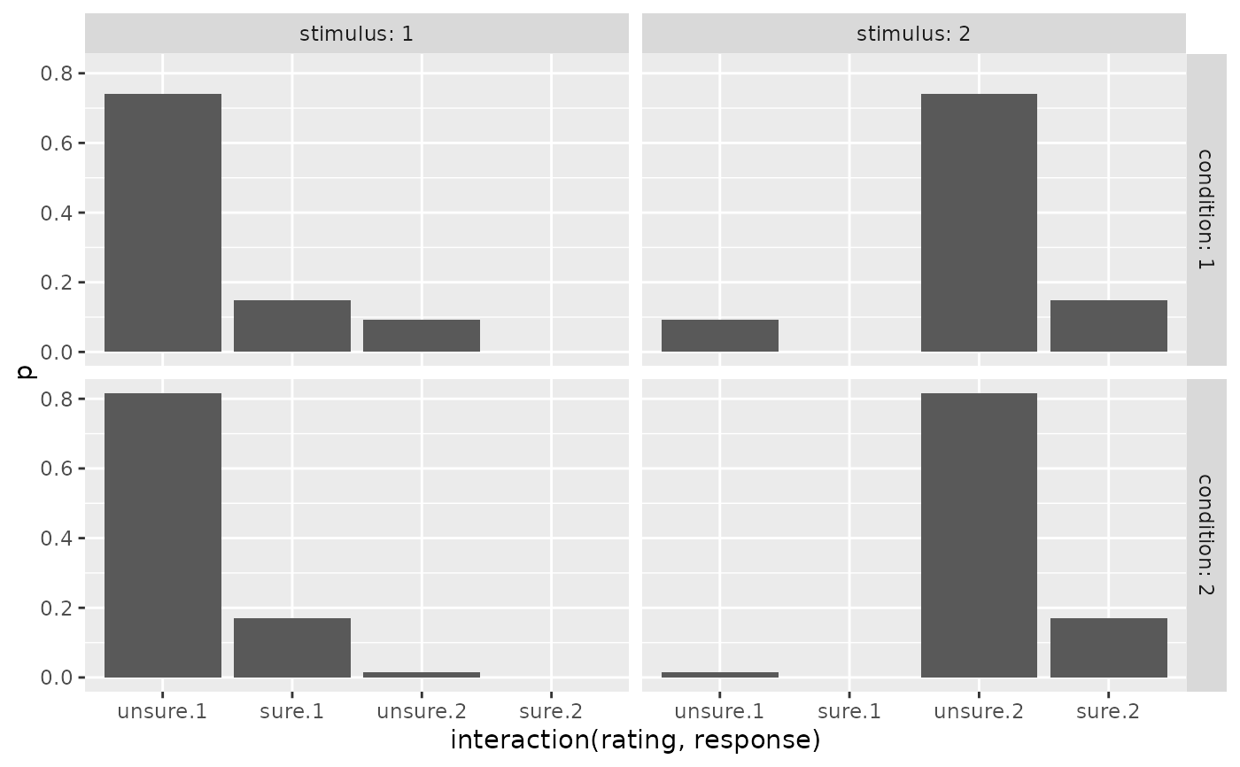
preds_Conf$rating <- factor(preds_Conf$rating, labels=c("unsure", "sure"))
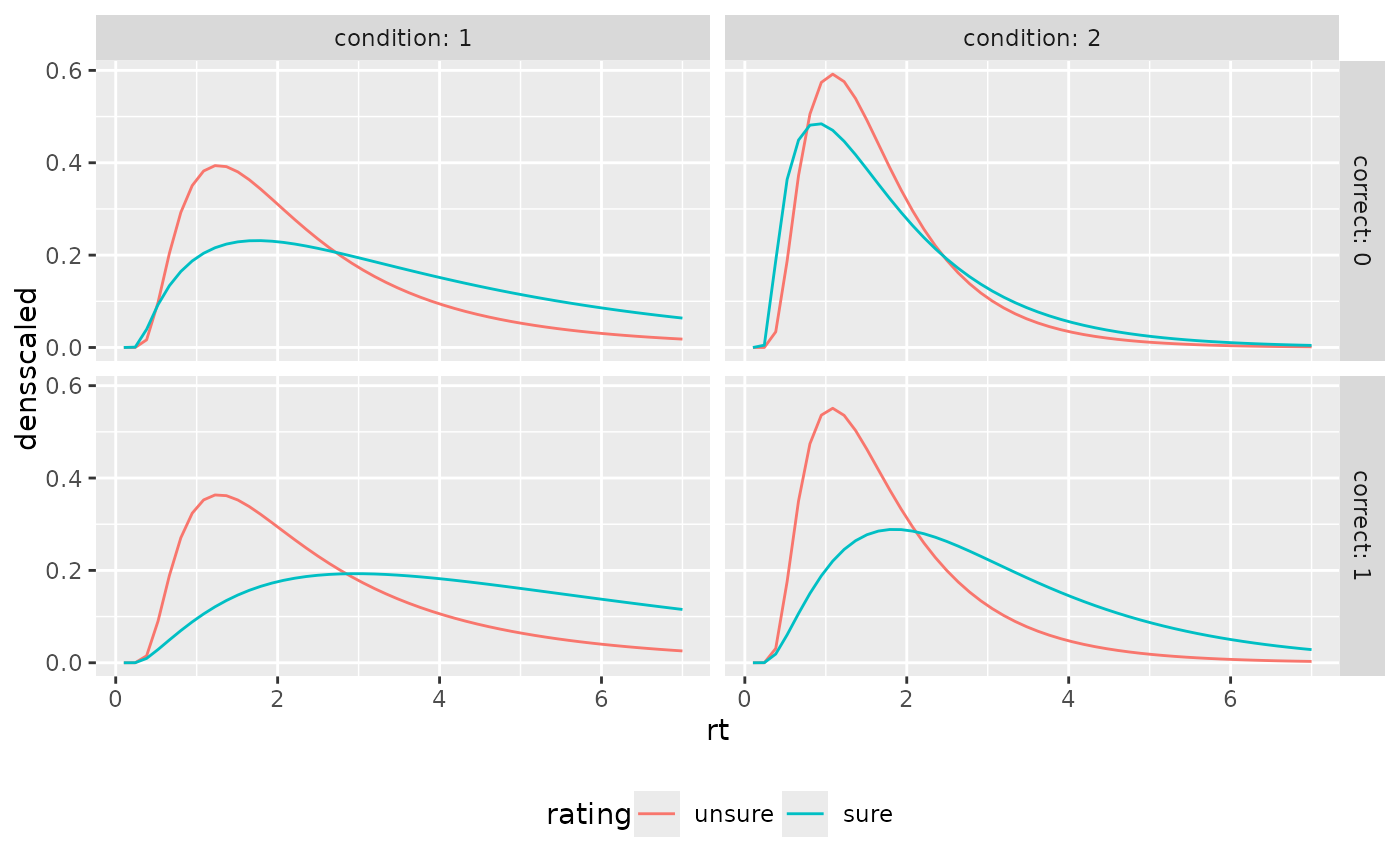
preds_RT$rating <- factor(preds_RT$rating, labels=c("unsure", "sure"))
ggplot(preds_Conf, aes(x=interaction(rating, response), y=p))+
geom_bar(stat="identity")+
facet_grid(cols=vars(stimulus), rows=vars(condition), labeller = "label_both")
 ggplot(preds_RT, aes(x=rt, color=interaction(rating, response), y=dens))+
geom_line(stat="identity")+
facet_grid(cols=vars(stimulus), rows=vars(condition), labeller = "label_both")+
theme(legend.position = "bottom")
ggplot(preds_RT, aes(x=rt, color=interaction(rating, response), y=dens))+
geom_line(stat="identity")+
facet_grid(cols=vars(stimulus), rows=vars(condition), labeller = "label_both")+
theme(legend.position = "bottom")
 ggplot(aggregate(densscaled~rt+correct+rating+condition, preds_RT, mean),
aes(x=rt, color=rating, y=densscaled))+
geom_line(stat="identity")+
facet_grid(cols=vars(condition), rows=vars(correct), labeller = "label_both")+
theme(legend.position = "bottom")
ggplot(aggregate(densscaled~rt+correct+rating+condition, preds_RT, mean),
aes(x=rt, color=rating, y=densscaled))+
geom_line(stat="identity")+
facet_grid(cols=vars(condition), rows=vars(correct), labeller = "label_both")+
theme(legend.position = "bottom")
 # }
# \donttest{
# Use PDFtoQuantiles to get predicted RT quantiles
# (produces warning because of few rt steps (--> inaccurate calculations))
PDFtoQuantiles(preds_RT, scaled = FALSE)
#> Warning: There are only 50 rows for at least one subgroup of the data set.
#> Consider refining the rt-grid for more accurate computations.
#> # A tibble: 80 × 7
#> condition stimulus response correct rating p q
#> <int> <dbl> <dbl> <dbl> <fct> <dbl> <dbl>
#> 1 1 1 1 1 unsure 0.1 0.945
#> 2 1 1 1 1 unsure 0.3 1.51
#> 3 1 1 1 1 unsure 0.5 2.07
#> 4 1 1 1 1 unsure 0.7 3.06
#> 5 1 1 1 1 unsure 0.9 4.75
#> 6 1 1 1 1 sure 0.1 1.51
#> 7 1 1 1 1 sure 0.3 2.63
#> 8 1 1 1 1 sure 0.5 3.76
#> 9 1 1 1 1 sure 0.7 4.89
#> 10 1 1 1 1 sure 0.9 6.16
#> # ℹ 70 more rows
# }
# }
# \donttest{
# Use PDFtoQuantiles to get predicted RT quantiles
# (produces warning because of few rt steps (--> inaccurate calculations))
PDFtoQuantiles(preds_RT, scaled = FALSE)
#> Warning: There are only 50 rows for at least one subgroup of the data set.
#> Consider refining the rt-grid for more accurate computations.
#> # A tibble: 80 × 7
#> condition stimulus response correct rating p q
#> <int> <dbl> <dbl> <dbl> <fct> <dbl> <dbl>
#> 1 1 1 1 1 unsure 0.1 0.945
#> 2 1 1 1 1 unsure 0.3 1.51
#> 3 1 1 1 1 unsure 0.5 2.07
#> 4 1 1 1 1 unsure 0.7 3.06
#> 5 1 1 1 1 unsure 0.9 4.75
#> 6 1 1 1 1 sure 0.1 1.51
#> 7 1 1 1 1 sure 0.3 2.63
#> 8 1 1 1 1 sure 0.5 3.76
#> 9 1 1 1 1 sure 0.7 4.89
#> 10 1 1 1 1 sure 0.9 6.16
#> # ℹ 70 more rows
# }